Optimizer 101
This section contains information about the workflow of the QDesignOptimizer (QDO).
Why QDO?
Tuning up a superconducting quantum chip often involves lengthy simulations where the user manually updates the design variables, such as capacitance lengths and Josephson junction sizes, to reach the parameter targets of the circuit, such as frequencies, decay rates and coupling strengths. The QDesignOptimizer package strongly reduces the need for manual intervention by automating the simulation and optimization of the design variables. The optimization cycle first runs a detailed and often time-consuming electro-magnetic Ansys HFSS simulation [1] combined with Energy Participation Ratio (EPR) analysis [2] to estimate the current values of the circuit parameters, integrated together with design framework Qiskit Metal [3]. The second step solves a nonlinear approximate model based on the user’s physical knowledge about the circuit, which estimates how the design variables should be changed to reach the target. The flexibility in the QDesignOptimizer setup allows for the efficient investigation of chip subsystems since the simulation and approximate physical model are dynamically compiled from the user settings.
QDO Concept
The optimization framework allows for a systematic and automated optimization of quantum chip designs based on physical models including:
Eigenmode simulations
Capacitance simulations
Energy participation ratio analysis
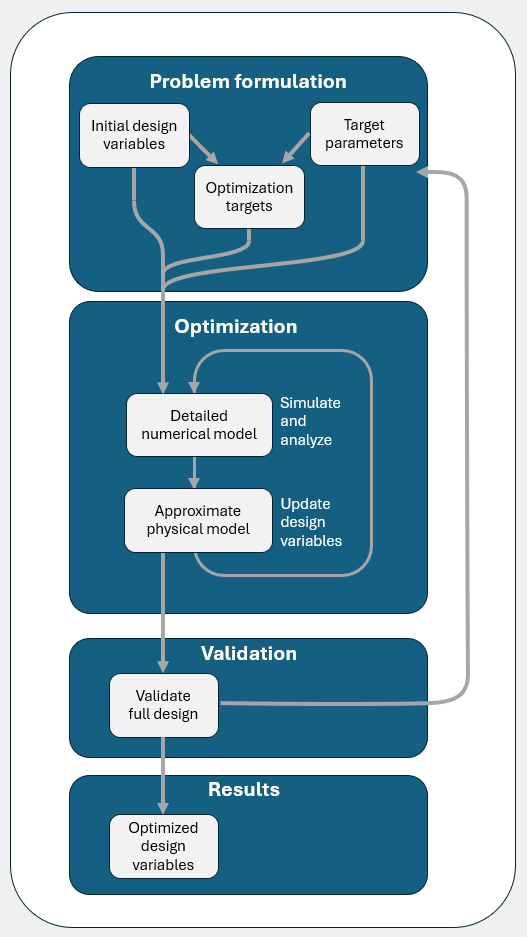
The workflow of the QDesignOptimizer follows a three-step logic, which is also shown in the figure below:
Problem formulation
Optimization based on physical models
Validation and results
In short, in the problem formulation the user specifies the parameter targets, an initial guess for the design variables, and the optimization targets holding the approximate physical relationships between the parameters and variables. The optimization step is an iterative process that begins with a detailed electromagnetic simulation and energy participation ratio analysis for the current design variables, which provide the current values of the parameters. The approximate nonlinear model specified in the optimization targets is then solved, suggesting a good approximation to the optimal design variables, leading to convergence after a few iterations. | Further information on the setup can be found in User Guide.
Problem Formulation
The general idea is to identify \(N\) design variables \(\overrightarrow{V}=\{V_1, ..., V_N\}\), which can be varied so that the targets of the \(N\) parameters \(\overrightarrow{Q}=\{Q_1, ..., Q_N\}\) can be reached. These definitions are done by setting up one Optimization Target for each parameter, which specifies the physical, generally nonlinear relation of how the parameter depends on the varying design variables as well as (other) parameters, i.e.,
As an initial guess for the optimization, the user will provide sensible values for the design variables \(\overrightarrow{V}\).
Simulate Design Variables
To obtain knowledge of which values of the parameters the current design variables result in, the QDesignOptimizer runs a detailed electromagnetic simulation (by choice an eigenmode and/or capacitance simulation) in Ansys HFSS and performs an energy-participation ratio (pyEPR) analysis. The parameters \(\overrightarrow{Q}^{k}\), in the k-th iteration, are then extracted from the simulation and analysis results.
Update Design Variables
In update step number \(k\), the optimizer updates the design variables from the ones used in the simulation \(\overrightarrow{V}^{k}\) to \(\overrightarrow{V}^{k+1}\), such that \(\overrightarrow{Q}_i^{k+1}\) gets close to the target value \(Q_i^{target}\). Due to the assumption of proportionality between \(Q_i\) and \(F_i\), the updated parameter is estimated as:
Note that we here distinguish between the parameter \(\overrightarrow{\tilde Q}\) estimated by the approximate model and the simulated parameter \(\overrightarrow{Q}\), which is typically more accurate. The more accurate the physical model is, which we set up in the equation above, the smaller is the discrepancy \(|| \overrightarrow{Q}- \overrightarrow{\tilde Q}||\), and the faster the optimization converges.
To obtain the updated design variables \(\overrightarrow{V}^{k+1}\), the QDesignOptimizer minimizes the cost function:
by finding the optimal \(\overrightarrow{V}^{k+1}\). If the problem is correctly formulated, the minimization will reach \(\tilde Q_i^{k+1} = Q_i^{target}\) for all \(i=1,...,N\) targets in the optimization. However, the QDesignOptimizer assumes that parameters, which are not associated with an Optimization Target, will not be affected by the changed design variables, i.e., \(\tilde Q_i^{k+1} = Q_i^{k}\) for \(i>N\), if the system contains more parameters than targets.
These relations for \(\tilde Q_i^{k+1}\) simplify parameter updates to only depend on:
The values of the parameters in the previous step,
The target values, and
The design variables.
One of the main assumptions, which the QDesignOptimizer takes advantage of is that, if the approximate model incorporates the correct general trends of the physical relationships, the optimization will converge to the target. Hence, there is no need for the user to specify a very precise physical model, but the more the user knows about the physics, the faster and more robust the optimizer will be.
Separating physical dependencies by design
Independent Variables
The number of independent design variables \(N\) must match the number of parameters that have a target in the optimization. In the example discussed in QDO QuickStart, we consider the \(N=5\) parameters specified in table under Physical relation, where the corresponding five design variables are:
Resonator length \(l_{res}\)
Qubit Josephson junction inductance \(L_{qb}\)
Qubit width \(w_{qb}\)
Resonator-qubit coupling width \(w_{res-qb}\)
Resonator to transmission line coupling length \(l_{res-tl}\)
Factorization of Update Step
The resonance frequency of the resonator \(f_{res}\) depends solely on the resonator length \(l_{res}\)
The coupling of the resonator to the feedline \(\kappa_{res}\) depends solely on the resonator to feedline coupling length \(l_{res-tl}\)
The qubit capacitance energy \(f_{qb}\) is influenced only by the qubit width \(w_{qb}\).
Instead of minimizing all parameters simultaneously, the optimizer first solves the following one-dimensional optimization problems to obtain the updated design variables:
Determine \(l_{res}^{k+1}\) by minimizing the cost function with respect to \((f_{res}, l_{res})\).
Determine \(l_{res-tl}^{k+1}\) by minimizing the cost function with respect to \((\kappa_{res}, l_{res-tl})\).
Determine \(w_{qb}^{k+1}\) by minimizing the cost function with respect to \((f_{qb}, w_{qb})\).
Once these one-dimensional optimizations are complete, we solve the remaining two-dimensional problem involving:
Determine \(\chi_{qb-res}^{k+1}\) by solving for \((f_{qb}, \chi, L_{qb}, w_{res-qb})\)
Footnotes